
Computation Graph Optimization 2부 - 모델 추론 속도를 위한 그래프 구조 정리법
LLM 추론 속도를 극대화하는 고급 그래프 최적화 기법 총정리. FP16, INT8, 커널 퓨전 등 실전 적용 전략을 사례와 함께 소개합니다.
이전 글에서는 Computation Graph의 개념과 기초 최적화 기법에 대해 살펴봤습니다. 이번 글은 그에 이은 두 번째 글로, 보다 실전적인 최적화 전략을 담고 있습니다.
- 이번 Part 2에서는 정밀도 축소, 실행 그래프 최적화, Transformer 구조 특화 기법 등 실시간 추론 성능 향상에 핵심적인 기법들을 소개합니다.
- 먼저 업로드된 Part 1(Computation Graph Optimization 1부 - 최적화의 출발점)을 함께 참고하시면 더욱 좋습니다.
- 이 글은 올거나이즈 RAG팀의 조한준 엔지니어님이 작성하셨습니다.
4. Computation Graph Optimization Frameworks
4.1 Overview of Optimization Frameworks
Computation graph 최적화는 추론 속도를 높이고 자원 효율성을 극대화하는 데 있어 핵심적인 역할을 합니다.
이를 위해 다양한 최적화 프레임워크가 등장했으며, 각 프레임워크는 서로 다른 graph 표현 방식, 최적화 전략, 실행 backend를 기반으로 동작합니다.
4.1.1 최적화 프레임워크의 주요 기능
- 연산자 수준에서 fusion, folding, elimination 등 다양한 최적화 패스 적용
- tensor의 shape, layout, precision을 정적으로 확정하거나 재구성
- target backend에 최적화된 실행 계획(execution plan) 생성
- dynamic graph를 static graph로 변환하거나, runtime 시점에서 graph specialization 수행
4.1.2 대표적인 최적화 프레임워크
4.1.3 적용 시점 기준 정리
각 프레임워크의 적용 시점은 최적화 방식과 대응 가능한 환경에 큰 영향을 미칩니다.
예를 들어 TensorRT는 build-time 최적화에 특화되어 있는 반면, TorchDynamo나 ONNXRuntime EP는 runtime 시점에서도 유연한 graph 변형이 가능합니다.
4.1.4 프레임워크 선택 시 고려 요소
- 모델의 graph 구조 (static vs dynamic)
- 타겟 환경 (GPU, CPU, edge 등)
- 최적화 강도 (conservative vs aggressive)
- ecosystem 통합성 (PyTorch-native, ONNX-compatible, CUDA-specific 등)
실제 서비스에 적용할 경우, 이들 프레임워크의 조합을 통해 최적화 범위를 확장하는 것도 하나의 전략이 될 수 있습니다.
예를 들어 PyTorch → ONNX export → TensorRT 빌드까지의 파이프라인을 구성하면, 학습 환경의 유연성과 추론 환경의 성능을 모두 확보할 수 있습니다.
4.2 TorchScript
TorchScript는 PyTorch 모델을 static computation graph로 변환하여 Python 없이 추론 가능한 형태로 만드는 중간 표현입니다.
Triton Inference Server에서 PyTorch 모델을 배포할 때 가장 널리 사용되는 표준 포맷이기도 합니다.
4.2.1 Graph 구조 및 동작 방식
TorchScript는 PyTorch 모델을 ScriptModule 또는 TracedModule로 변환해 static 연산 그래프 형태로 표현합니다.
내부적으로는 SSA(Static Single Assignment) 기반의 intermediate representation을 사용하며,
모델의 연산, tensor 흐름, 조건문 등을 모두 graph node로 변환합니다.
변환 방식은 두 가지입니다.
torch.jit.trace- 예시 입력의 forward 경로를 따라 연산을 기록
- Python control flow는 무시됨 (if, loop 등은 포함되지 않음)
torch.jit.script- Python 코드 자체를 파싱해 제어 흐름까지 포함한 static graph 생성
- 함수 정의, 타입 주석 등 문법 제약이 있음
생성된 모델은 .pt 파일로 export 가능하며,
Python runtime 없이 C++(LibTorch) 혹은 Triton Server에서 직접 실행할 수 있습니다.
4.2.2 지원 최적화 기법
TorchScript는 static graph 상에서 기본적인 최적화를 자동으로 수행합니다.
최적화 강도는 보수적인 편이지만, Python-free 추론 환경 구성에 매우 적합합니다.
4.2.3 장점과 한계
장점
- Python 없이 추론 가능 (Triton, C++, 모바일 등)
- PyTorch-native 모델을 별도 프레임워크 없이 export 가능
- 정적 graph로 memory plan, shape 고정 등 최적화 가능
- Triton에서
.pt포맷을 그대로 배포 가능
한계
trace방식은 dynamic control flow를 반영하지 못함script방식은 Python 문법 제약이 많음- low-level memory layout, kernel tuning은 미지원
- export 실패 시 debug 경험이 불편함
- 정적 양자화는 실질적으로 지원되지 않음
4.2.4 Triton Inference Server에서의 활용
TorchScript는 Triton Inference Server의 PyTorch backend에서
공식 지원하는 유일한 static graph 포맷입니다.
기본 적용 흐름
- PyTorch로 모델 학습 및
.eval()전환 torch.jit.trace()또는torch.jit.script()로 graph export.pt파일을model_repository/my_model/1/에 저장config.pbtxt에서 backend를pytorch_libtorch로 지정
실전 활용 팁
- TorchScript +
optimize_for_inference()→ Dropout 제거, Folding 적용 - TorchScript + FP16 export → Tensor Core 활용 가능
- TorchScript + Ensemble 구성 → 전처리/후처리 모델과 조합
4.2.5 TorchScript Export 코드 예시
4.2.6 TorchScript 최적화 및 FP16 적용
FP16 추론을 Triton에서 사용하려면 config.pbtxt의 input/output 타입을 TYPE_FP16으로 설정해야 합니다.
4.3 ONNX
ONNX(Open Neural Network Exchange)는 PyTorch, TensorFlow, MXNet 등 다양한 프레임워크에서
학습된 모델을 하나의 공통 포맷으로 export하고 추론 환경에 최적화할 수 있도록 설계된 중간 표현(IR)입니다.
ONNX는 추론 중심의 static graph 기반 구조를 사용하며,
ONNX Runtime, TensorRT, OpenVINO 등 다양한 backend에서 동일한 모델을 실행할 수 있습니다.
4.3.1 Graph 구조 및 동작 방식
ONNX는 static computation graph 형식으로 모델을 표현합니다.
모델 구조와 weight는 export 시점에 완전히 고정되며, Python 없이 실행 가능한 형태로 변환됩니다.
PyTorch에서는 torch.onnx.export()를 통해 ONNX 모델을 생성하며,
내부적으로 tracing 방식으로 연산 그래프를 기록합니다.
생성된 .onnx 파일은 ONNX IR(GraphProto) 형식이며,
ONNX Runtime, TensorRT, OpenVINO 등 다양한 추론 엔진에서 바로 로드해 실행할 수 있습니다.
4.3.2 지원 최적화 기법
ONNX는 static graph 기반이기 때문에 다양한 최적화 기법을 적용할 수 있습니다.
ONNX 자체 optimizer 외에도 ONNX Runtime, TensorRT, GraphSurgeon 등에서 backend-specific 최적화가 추가로 적용됩니다.
4.3.3 장점과 한계
장점
- 다양한 프레임워크 간 모델 호환성 확보 (PyTorch, TensorFlow 등)
- ONNX Runtime, TensorRT, OpenVINO 등 여러 backend 지원
- 정적 quantization, FP16 변환 등 추론 중심의 최적화 지원
- CPU, GPU, Edge 환경 모두 대응 가능
한계
- tracing 기반이므로 dynamic control flow 표현에 제약 있음
- PyTorch to ONNX 변환 시 aten:: 연산자 → onnx:: mapping 문제가 발생할 수 있음
- custom kernel, weight sharing 등 일부 구조는 변환이 어렵거나 누락됨
- export 오류 발생 시 debug 난이도 높음
4.3.4 Triton Inference Server에서의 실전 활용
ONNX는 Triton Inference Server에서 가장 널리 사용되는 모델 포맷 중 하나입니다. onnxruntime 또는 tensorrt backend를 통해 GPU/CPU에서 추론을 실행할 수 있습니다.
실전 적용 흐름
torch.onnx.export()로 ONNX 모델 생성model_repository/my_model/1/model.onnx에 저장config.pbtxt에서 backend를onnxruntime또는tensorrt로 설정- Triton이 static graph를 로드하여 추론 서비스 제공
Backend 선택 가이드
추가 최적화 도구
onnxsim– 불필요한 노드 제거 및 shape 고정onnxruntime_tools,onnx-graphsurgeon– 수동 최적화- TensorRT builder – precision별 engine 생성 (FP16, INT8)
4.3.5 ONNX Export 코드 예시
4.3.6 ONNX 모델 간소화 (onnx-simplifier)
4.3.7 Triton config 예시
4.3.8 ONNX Static Quantization (INT8)
4.4 TensorRT
TensorRT는 NVIDIA에서 제공하는 고성능 딥러닝 추론 최적화 라이브러리입니다.
FP16, INT8, layer fusion, kernel auto-tuning 등의 최적화를 통해 GPU 상에서 최소 latency, 최대 throughput을 달성하는 것이 목적입니다.
PyTorch, ONNX, TensorFlow 모델을 입력으로 받아
CUDA-compatible static inference engine (.plan 파일)으로 변환하여 추론을 수행합니다.
4.4.1 구조 및 최적화 파이프라인
TensorRT는 모델 최적화를 다음과 같은 세 단계로 구성합니다:
- Graph Parsing
- ONNX 모델을 로드하여 내부 graph IR로 변환
- Tensor, shape, op dependency 등 정보 추출
- Graph Optimization
- Layer Fusion, Constant Folding, Dead Code Elimination 등 적용
- Precision 전환 (FP32 → FP16/INT8), Layout 최적화 수행
- Engine Building
- CUDA kernel 기반으로 layer별 최적 실행 계획 수립
- Shape, batch size, precision이 고정된
.plan파일 생성
4.4.2 지원 최적화 기법
TensorRT는 다음과 같은 고수준 최적화 패스를 지원합니다.
4.4.3 Engine 구성 및 저장
TensorRT는 .plan 파일 형식의 static engine을 생성합니다.
이 파일은 최적화된 CUDA kernel, memory binding, shape profile을 포함하며, 추론 시 바로 실행할 수 있습니다.
Engine 설정 주요 항목
max_batch_size: 최대 배치 크기min/opt/max_shape: dynamic shape profile 정의precision_mode: FP16, INT8 설정workspace_size: GPU 메모리 사용 한도
Python, C++, CLI(trtexec) 등 다양한 방법으로 엔진을 생성할 수 있습니다.
4.4.4 Triton Inference Server 연동
Triton에서 TensorRT .plan 파일을 사용하려면 platform: "tensorrt_plan"을 지정합니다.
실전 적용 흐름
- ONNX 모델 export
- TensorRT builder로 최적화된
.plan생성 model_repository/my_model/1/model.plan에 저장config.pbtxt에 precision, shape profile 등 설정- Triton 서버 시작 → 자동 로딩 및 추론 제공
INT8 사용 시
- Calibration cache(
calib.cache) 파일을 함께 제공하면 재학습 없이 deployment 가능
4.4.5 장점과 한계
장점
- GPU 성능 최적화 수준이 가장 높음
- Layer fusion, precision 변환, memory plan 등 자동 적용
- 다양한 shape profile 지원으로 runtime 유연성 확보
- PyTorch, TensorFlow, ONNX 등 다양한 input 포맷 지원
한계
- 엔진 생성 복잡, 빌드 시간 길고 GPU 환경 종속
- Dynamic shape은 profile에 명시된 범위만 지원
- CUDA driver, GPU 종류가 바뀌면 재빌드 필요
- 엔진이 proprietary binary → 재현성과 이식성 제약 있음
4.4.6 TensorRT Python API 예시
4.4.7 INT8 Calibration 적용
4.4.8 Triton config.pbtxt 예시
4.4.9 trtexec CLI 활용 예시
5. Latency Optimization Result in Enterprise-Scale System
Transformer 기반 임베딩 시스템에서 실시간 추론 속도 개선을 위해 하드웨어 교체, 정밀도 축소, 그래프 최적화를 적용했습니다.
Token 길이에 따른 latency 구성 요소를 분석하고, 각 최적화 단계가 실제 성능에 미치는 영향을 정량적으로 보고합니다.
5.1 실험 설정
- 대상 모델: BAAI/bge-m3
- Task: 단일 문서 임베딩 추론
- 입력 길이: 64 ~ 8192 tokens
- 최대 입력 길이: 4096 tokens
- 실행 환경: Triton Inference Server + (TensorRT, ONNX, TorchScript)
- GPU: NVIDIA T4 (baseline) → NVIDIA L4
- Precision: FP32 → FP16
- Benchmark 방식: Per-document latency 측정 (batch=1)
5.2 최적화 단계 구성
- 색상 구분:
- 빨간색: L4 + FP32
- 연두색: L4 + FP16
- 하늘색: 최종 최적화 버전 (FP16 + Graph Optimization)
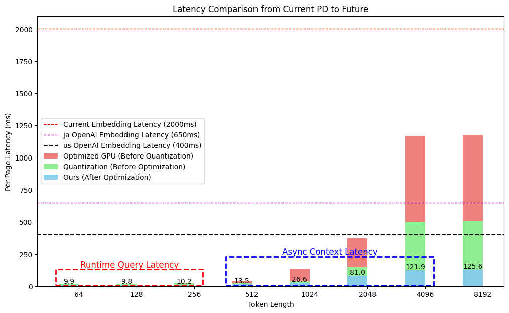
5.3 Token 길이별 분석 요약
- 4096 token 기준:
- FP32: 약 1200ms
- FP16: 약 550ms
- FP16 + Graph 최적화: 약 120ms
5.4 적용된 최적화 기법 요약
FP16 기반 정밀도 축소
- 전체 연산 FP16 처리
- LayerNorm 및 Softmax는 FP32 유지
- PyTorch AMP 및 TensorRT builder 기반 precision pass 활용
Computation Graph 최적화
- Operator Fusion (Linear + Add + GELU + LayerNorm)
- Memory Reuse (중간 tensor buffer 재활용)
- Transpose Elimination (불필요한 layout 전환 제거)
- Common Subexpression Elimination (mask, embedding 공유)
- Dead Code Elimination (Dropout 등 제거)
- Weight Sharing 및 Buffer Folding
5.5 OpenAI Embedding API와 비교
- Runtime Query 기준: OpenAI 대비 30~50배 빠른 Latency
- Async Context 기준: OpenAI 대비 3~5배 빠른 Latency
Baseline(비 최적화)은 Fixed Length 방식으로 항상 max_token_length의 지연시간을 요구했으나, Variable Length를 지원하면서 적은 토큰 수에서 latency가 수백 배 이상 개선되었습니다.
특히 runtime latency가 중요한 Query의 경우 토큰 수가 적기 때문에 향상 폭이 매우 큰 것이 핵심입니다. Graph 최적화를 통해 Async Context Latency도 수십 배 이상 개선되었습니다.
5.6 Reranker (Cross-Encoder) Latency 비교: 10개 고객사 데이터셋
고객사 데이터를 대상으로 Reranker 모델의 속도를 static graph 최적화를 통해 개선한 실험 결과입니다.
정확도는 거의 동일하거나 유지되었으며, 평균적으로 1.33배 빠른 latency 개선이 확인되었습니다.
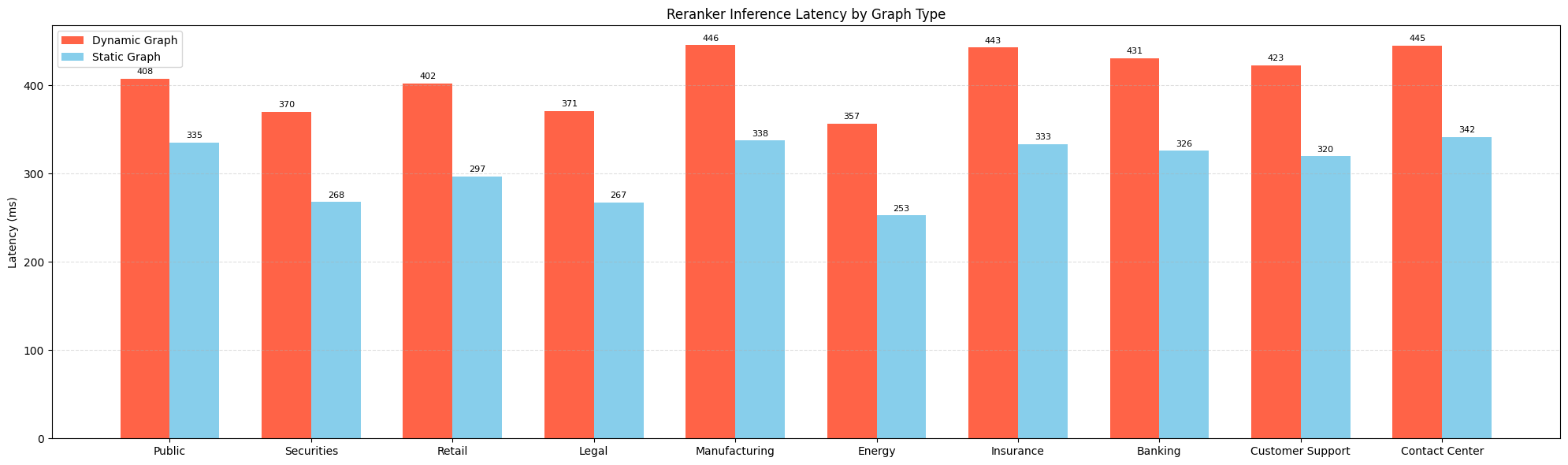
대부분 케이스에서 정확도 유지 혹은 소폭 향상
평균적으로 latency 1.33배 개선
특히 300ms 이상 응답 시간이 발생하는 기업 환경에서 체감 성능 개선 효과가 명확
5.6 실전 적용 시 고려사항
Precision 관련
- LayerNorm, Softmax는 FP16 rounding error에 민감 → FP32 유지 필요
- A100, L4 등 mixed precision 지원 GPU에서 FP16 효과 극대화 가능
Memory 관리
- 2048 token 이상에서는 activation memory가 병목 → memory reuse 병행 최적화 필요
배포 측면
- 4096~8192 token 기준 latency 150ms 이내 확보 → OpenAI 대체 가능한 실시간성 도달
5.7 최적화 결과 요약
- 단순한 하드웨어 교체(T4 → L4)만으로는 충분한 latency 개선이 어려움
- A100, H100 수준의 고가 GPU는 상업 환경에서는 가격 경쟁력에서 한계 존재
- FP16 정밀도 축소 + Computation Graph 최적화 병행 시, 긴 문서에서도 실시간 응답 시간 확보 가능
- 특히 1024 token 이상 구간에서 graph-level 최적화의 latency 감소 효과가 뚜렷하게 관찰됨
- 실험 결과, 4096 token 기준 기존 시스템 대비 16배 빠른 추론, OpenAI 대비 최대 5배 개선 효과 확인됨
5.8 Embedding Model 비교 성능 분석
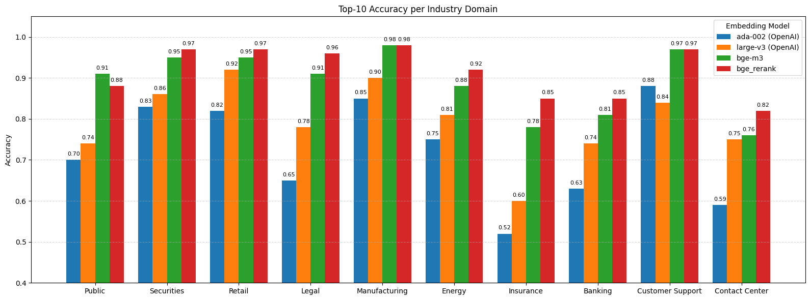
저희가 자체 보유한 산업 도메인별 데이터를 기반으로 다양한 embedding 모델의 성능을 비교한 결과입니다.
모델 설명
- ada-002: OpenAI에서 제공했던 구세대 임베딩 모델
- large-v3: 현재 OpenAI API에서 제공하는 최상위 embedding 모델
- bge-m3: 자체적으로 서빙 중인 BAAI/bge-m3 모델, 공개 모델 중 SOTA 성능
- bge_rerank: bge-m3에 cross-encoder reranker를 추가한 조합
주요 결과
- 대부분의 도메인에서 bge-m3 모델은 기존 OpenAI 모델 대비 월등한 Top-10 정확도를 기록함
- bge_rerank는 모든 도메인에서 가장 높은 정확도를 기록. 특히 어려운 도메인 (법률, 금융)에서 강세
- OpenAI 모델 간에도 성능 차이가 있으며, 전반적으로 bge-m3 대비 10~20% 낮은 정확도
결론 및 도입 효과
- 성능: bge-m3 모델의 도입으로 기존 OpenAI embedding 대비 최대 20% 정확도 향상
- 속도: 내부 최적화를 통해 OpenAI API 대비 30~50배 빠른 latency 확보
- 단가 절감: 자체 서빙을 통해 외부 API 사용 없이 embedding 코스트를 대폭 절감
이러한 성능-속도-비용 균형은 실시간 질의 대응이 중요한 산업 현장에서 중요한 경쟁력으로 작용하며,
특히 1024 token 이상의 긴 문서 처리에 있어서도 유리한 응답성을 확보할 수 있습니다.
6. 결론: 실시간 RAG 시스템을 위한 추론 최적화 전략
RAG 시스템의 실시간 응답 성능은 결국 Transformer 기반 모델의 추론 효율성에 의해 좌우됩니다. 특히 cross-encoder 기반의 reranker는 문서 수에 따라 연산량이 선형 증가하기 때문에, per-query latency의 병목 지점으로 작용하기 쉽습니다.
이번 프로젝트에서는 PyTorch 기반 모델을 static computation graph로 변환하고, 연산 구조, 데이터 흐름, 메모리, 정밀도, Transformer 구조 특화 등 다각도의 최적화 기법을 체계적으로 적용해보았습니다.
정적 최적화: 구조에서 출발한 변화
Linear + Add + LayerNorm을 하나의 fused kernel로 통합하거나, Q/K/V projection을 하나의 연산으로 병합하는 Operator Fusion은 kernel 호출 횟수를 줄이고 launch overhead를 줄여주는 핵심 기법이었습니다.
또한 Transpose Elimination, Common Subexpression Elimination, Dead Code Elimination 등 그래프 수준의 불필요한 흐름을 정리하면서 중간 tensor 이동을 줄이고, 더 나은 메모리 재사용 패턴을 확보할 수 있었습니다.
이와 함께 FP16 기반 정밀도 축소를 통해 전체 tensor 크기를 줄이고 Tensor Core를 활용한 연산 속도 향상을 달성했습니다. 단, LayerNorm이나 Softmax처럼 수치적으로 민감한 연산은 FP32로 유지하여 안정성도 확보했습니다.
Transformer에 특화된 최적화도 핵심
Transformer 모델은 그 자체로 반복 구조가 뚜렷한 모듈형 설계이기 때문에, Fused Multi-Head Attention, Rotary Embedding Precomputation, Key/Value Caching 같은 특화된 최적화 기법이 매우 효과적으로 작동합니다. 이들 기법은 특히 long-context inference 환경에서 memory reuse와 latency를 동시에 개선할 수 있는 핵심 도구입니다.
Framework 조합으로 실전 성능 극대화
모델 최적화는 결국 어떤 프레임워크 조합을 쓰느냐에 따라 달라집니다.
- TorchScript: PyTorch-native 환경에서 Python runtime 제거, 경량 실행 가능
- ONNX: 다양한 backend와 호환되는 유연한 구조, export 및 그래프 분석에 용이
- TensorRT: NVIDIA GPU에서 최상의 성능, kernel-level 최적화 및 precision scheduling 내장
특히 ONNX → TensorRT 경로를 활용하면 static graph 기반 구조에서 kernel-level 최적화와 precision tuning을 모두 적용할 수 있어, 엔터프라이즈 환경에서도 실용성과 효율성을 동시에 만족할 수 있습니다.
실험으로 확인된 효과
4096 token 기준:
- 기존 T4 + FP32 구조: 평균 latency 약 1200ms
- L4 + FP16 + Graph Optimization 구조: 평균 latency 약 121ms
즉, 10배 이상의 latency 개선을 확인했습니다.
또한 OpenAI Embedding API와 비교해도 최대 5배 빠른 응답 속도를 확보했습니다.
마무리하며
모델 최적화는 단순한 연산 속도 향상을 넘어, 실환경에서의 응답 성능과 안정성 확보를 위한 중요한 과정입니다. 이번 프로젝트를 통해 우리는 static computation graph 기반의 다양한 최적화 기법이 Transformer 모델의 추론 효율을 실질적으로 개선할 수 있음을 확인했습니다.
아직도 개선할 여지는 많습니다. 하지만 이러한 시도를 통해 점진적으로 시스템을 최적화해 나간다면, 실시간 RAG 시스템의 품질과 사용자 경험 모두를 향상시킬 수 있으리라 기대합니다.
우리 회사에 최고 성능의 LLM을 도입하고 싶다면 '올거나이즈'에 문의하세요!